Coming soon
Alley
Reflective ground, moving geometry
1Trinity College Dublin · 2Dolby Laboratories
Accepted to Pacific Graphics 2026
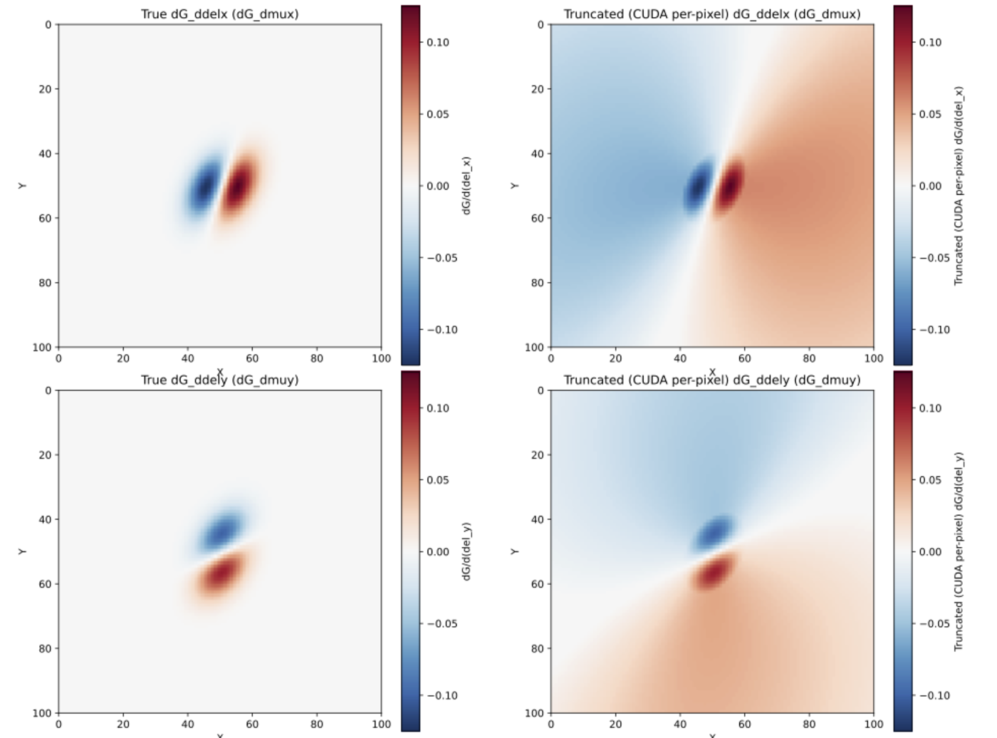
3D Gaussian Splatting has become a de facto scene representation for novel view synthesis, yet robustly learning 3D Gaussian primitives from visual input remains challenging. Standard optimization relies on gradient-based updates, but a common issue is the gradient vanishing phenomenon: a pixel far from a Gaussian primitive often has diminishing gradient magnitudes to influence primitive attributes, resulting in suboptimal scene reconstruction. In this paper, we propose a method to address gradient vanishing with a piecewise truncated gradient formulation that improves the optimization stability and robustness to initializations. We show that our method consistently improves 3D Gaussian Splatting with random and COLMAP initializations while being generalizable across static and dynamic Gaussian Splatting. As a by-product, we also examine the limitations of current benchmarks for dynamic scenes, and introduce a novel dataset for benchmarking dynamic Gaussian Splatting using synthetic 3D scenes. We demonstrate the effectiveness of our method in both static and dynamic settings for the public benchmarks and our proposed dataset.
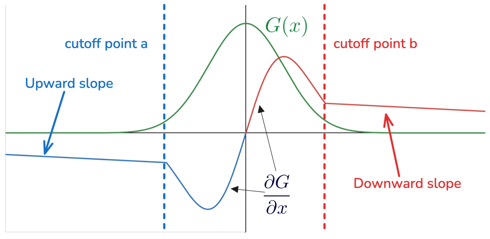
Keep the true Gaussian derivative inside the splat isocontour; continue it with a linear surrogate outside so distant pixels still move the primitive.
Cut-off \(\tau\) matches the rasterizer’s alpha discard; slope \(m\) sets far-field decay. Matching at \(x_b\) keeps the field continuous:
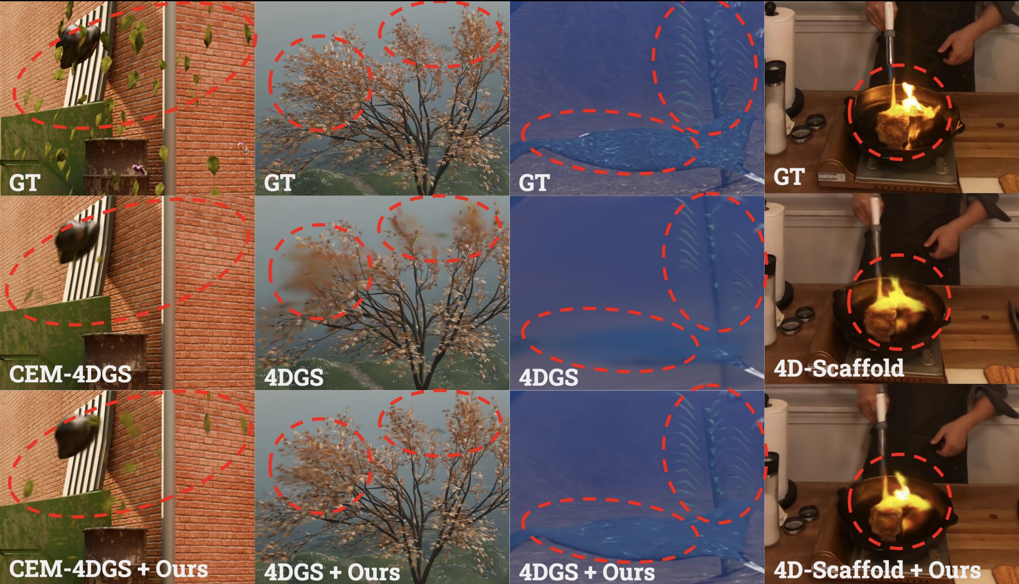
Drag across a clip to compare baseline vs. baseline + Ours. Clips load on demand.
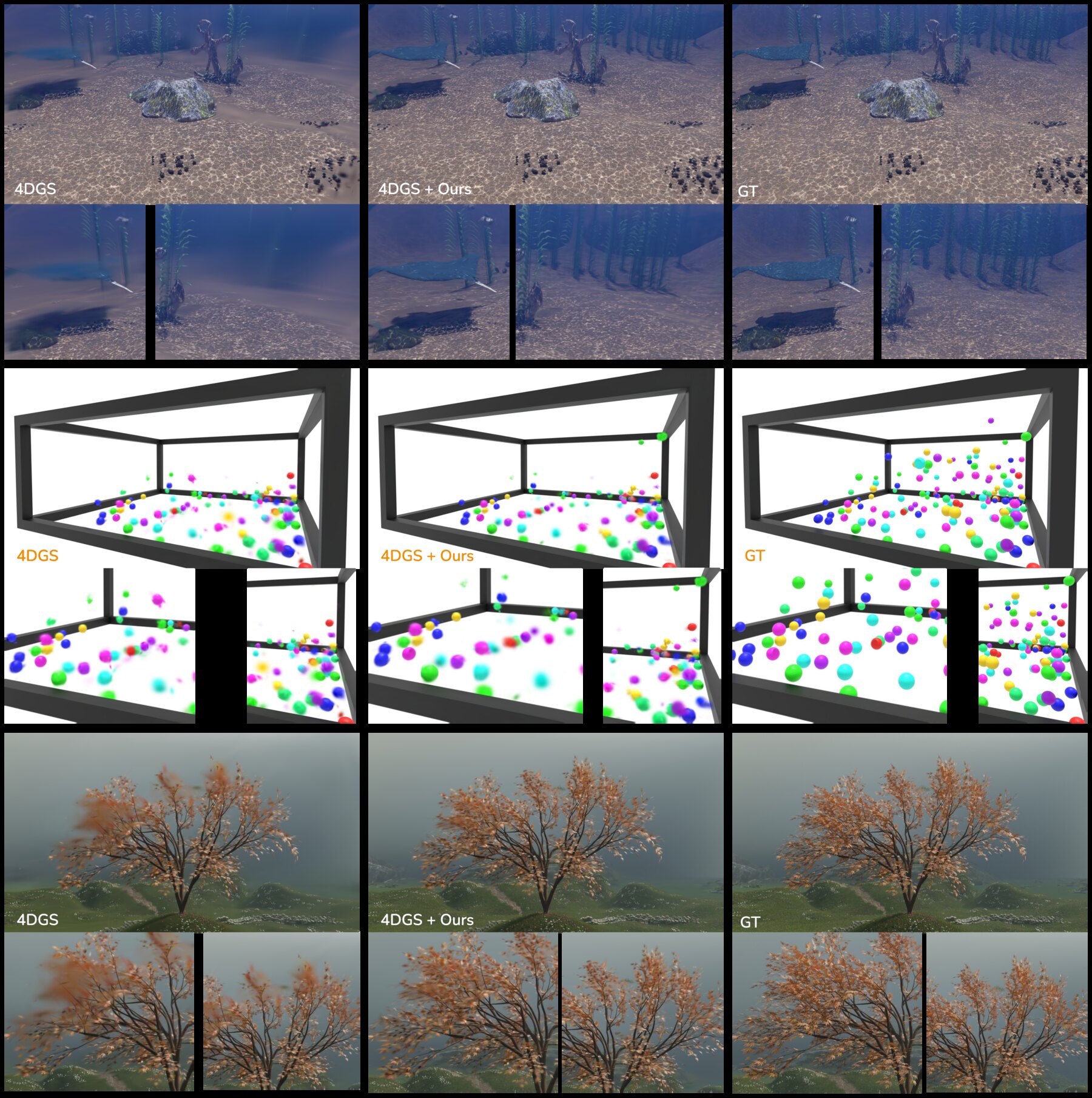
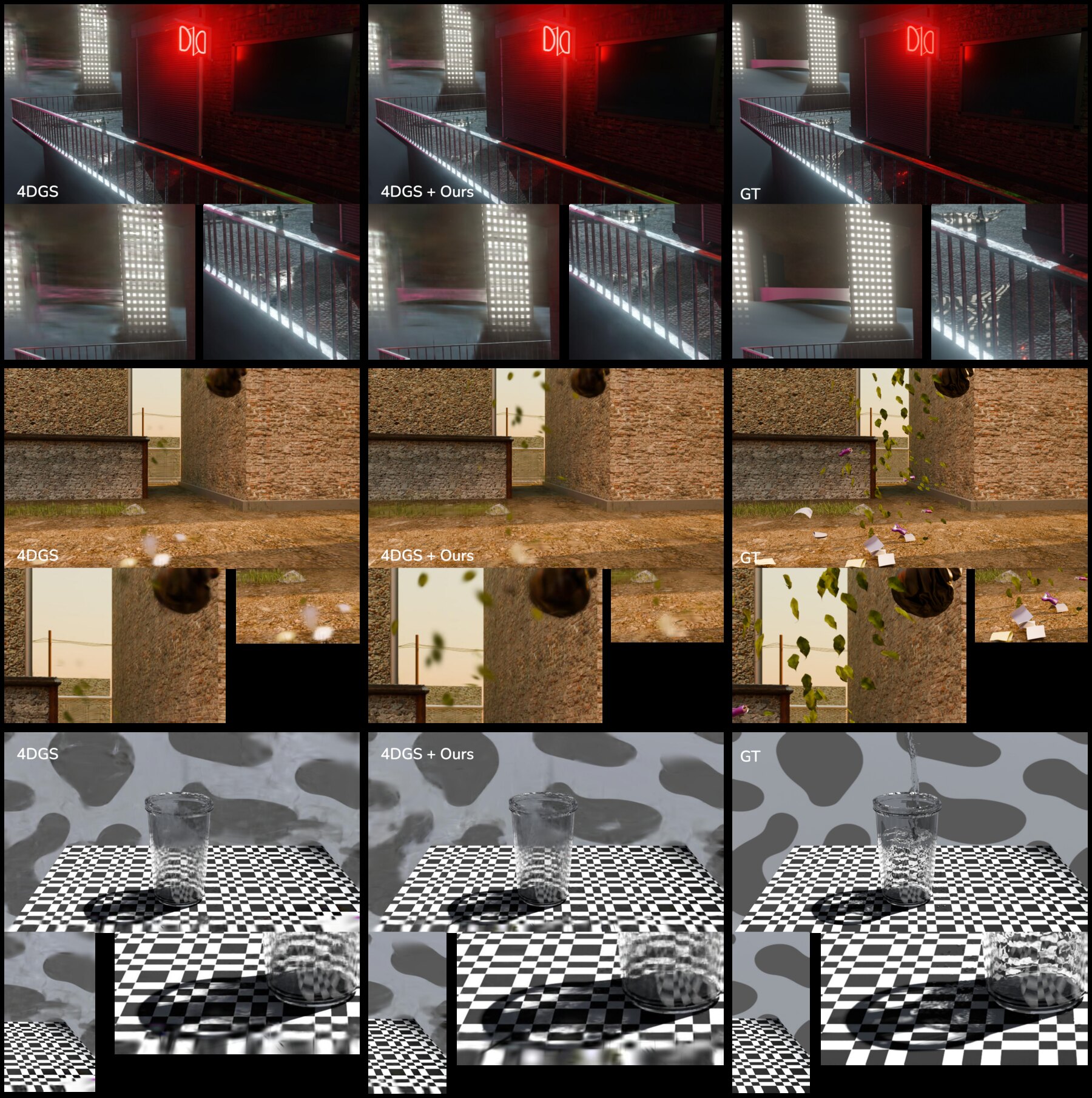
Six path-traced synthetic scenes with large spatio-temporal divergence — motion that public dynamic benchmarks rarely stress.
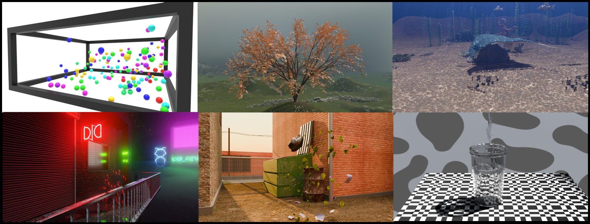
Reflective ground, moving geometry
Vegetation and outdoor atmospherics
Pouring fluid, caustics, refraction
Emissive night lighting
Sparse content, fast rigid motion
Volumetric scattering and fluid
Plug-in gains on Mip-NeRF360, Neural 3D Video, and our benchmark — better quality, often fewer Gaussians. Best per column in bold; our rows tinted.
Random and COLMAP init on OurBench and Mip-NeRF360. Train time is reference-only.
| Method | OurBench | Mip-NeRF360 | ||||||||
|---|---|---|---|---|---|---|---|---|---|---|
| LPIPS ↓ | SSIM ↑ | PSNR ↑ | Train ↓ | #GS ↓ | LPIPS ↓ | SSIM ↑ | PSNR ↑ | Train ↓ | #GS ↓ | |
| Random initialization | ||||||||||
| 3DGS | 0.2106 | 0.8351 | 24.74 | 14 min | 1.126M | 0.3481 | 0.6718 | 20.92 | 27 min | 1.180M |
| 3DGS + Ours | 0.1974 | 0.8511 | 25.16 | 55 min | 0.799M | 0.3343 | 0.6933 | 22.18 | 56 min | 0.971M |
| 2DGS | 0.4354 | 0.4960 | 18.80 | 23 min | 1.231M | 0.3943 | 0.6391 | 19.82 | 34 min | 1.511M |
| 2DGS + Ours | 0.3883 | 0.6624 | 20.70 | 33 min | 1.446M | 0.3886 | 0.6547 | 20.33 | 55 min | 1.071M |
| COLMAP initialization | ||||||||||
| 3DGS | 0.1270 | 0.9058 | 30.07 | 9 min | 1.217M | 0.2149 | 0.8212 | 27.70 | 21 min | 2.496M |
| 3DGS + Ours | 0.1245 | 0.9097 | 30.86 | 43 min | 0.768M | 0.2197 | 0.8205 | 27.84 | 86 min | 2.035M |
| 2DGS | 0.2017 | 0.8378 | 25.00 | 23 min | 1.801M | 0.2342 | 0.8117 | 27.17 | 44 min | 3.068M |
| 2DGS + Ours | 0.1962 | 0.8444 | 26.35 | 32 min | 1.048M | 0.2403 | 0.8104 | 27.33 | 80 min | 2.701M |
Sequential COLMAP init from the first frame. φ / θ = sparse / dense start on OurBench.
| Method | LPIPS ↓ | SSIM ↑ | PSNR ↑ | #GS ↓ |
|---|---|---|---|---|
| 4DGS | 0.1360 | 0.9443 | 30.22 | 2.806M |
| 4DGS + Ours | 0.1339 | 0.9493 | 31.70 | 1.733M |
| CEM-4DGS | 0.1328 | 0.9512 | 32.07 | 0.331M |
| CEM-4DGS + Ours | 0.1359 | 0.9519 | 32.29 | 0.352M |
| 4D-Scaffold | 0.1286 | 0.9502 | 31.83 | 0.583M |
| 4D-Scaffold + Ours | 0.1311 | 0.9487 | 31.94 | 0.556M |
| Method | LPIPS ↓ | SSIM ↑ | PSNR ↑ | #GS ↓ |
|---|---|---|---|---|
| 4DGS (φ) | 0.2326 | 0.8329 | 25.47 | 2.409M |
| 4DGS (φ) + Ours | 0.2035 | 0.8574 | 26.08 | 1.715M |
| 4DGS (θ) | 0.2288 | 0.8224 | 26.02 | 2.970M |
| 4DGS (θ) + Ours | 0.1496 | 0.8923 | 27.56 | 2.333M |
| CEM-4DGS | 0.2767 | 0.7855 | 22.80 | 0.704M |
| CEM-4DGS + Ours | 0.2670 | 0.7845 | 22.63 | 0.824M |
@inproceedings{morales2026truncgradgs,
  title        = {TruncGradGS: Improved 3D Gaussian Splatting via Truncated Gradient Updates},
  author       = {Morales, Th{\'e}o and Le-Pham, Nhat-Quynh and Atkins, Robin and Hua, Binh-Son},
  booktitle    = {Proceedings of Pacific Graphics 2026},
  year         = {2026},
  publisher    = {The Eurographics Association},
  eprint       = {2609.03534},
  archivePrefix = {arXiv},
  primaryClass = {cs.CV}
}